
The blog post explores the Poisson distribution, a statistical distribution commonly used in various fields, including astronomy, to model random events. It explains the properties of the distribution, its real-world applications, and provides a step-by-step guide on how to visualize the Poisson distribution using Python. The post also discusses the issue of Poisson noise in astronomical observations and presents a practical example of how to calculate and deal with it using Python.

The Poisson distribution is a probability distribution that models the number of rare events that occur in a fixed interval of time or space. It is widely used in many fields, including physics, biology, economics, and engineering. The distribution is named after the French mathematician Siméon Denis Poisson, who first introduced it in the early 19th century.
In this post, we will explore the Poisson distribution in detail, including its probability density function, mean, variance, and applications. We will also discuss Poisson noise and how we can model it using the Poisson distribution. Let’s get started!
What is the Poisson Distribution?
Poisson distribution is a discrete probability distribution that describes the probability of a given number of events occurring in a fixed interval of time or space. The distribution is often used to model rare events that occur randomly and independently of each other. The Poisson distribution has many practical applications, including modeling the number of traffic accidents in a given time period or the number of bacteria in a culture after a certain time.
The Poisson distribution is characterized by a single parameter, denoted by (lambda), which represents the mean number of events that occur in the given interval. The probability of observing events in the interval is given by the Poisson probability mass function (PMF):
where is the probability of events occurring in the interval, is the mathematical constant approximately equal to , and is the mean number of events.
The Poisson distribution has several important properties, including its mean and variance, which we will explore in the following section.
Mean and Variance of the Poisson Distribution
The mean, or expected value, of a Poisson distribution is denoted by , which represents the average number of events that occur in the given interval. It is also equal to the variance of the distribution.
The formula for the mean of a Poisson distribution is given by:
where denotes the expected value of the random variable .
The formula for the variance of a Poisson distribution is:
where denotes the variance of the random variable .
This means that the standard deviation of a Poisson distribution is:
The mean and variance of the Poisson distribution have important implications in many real-world applications. For example, if we know the average number of traffic accidents that occur in a certain area, we can use the Poisson distribution to estimate the probability of a certain number of accidents occurring in a given time period. Similarly, if we know the average number of customers that visit a store in a day, we can use the Poisson distribution to model the probability of a certain number of customers visiting the store in a given time period.
In the next section, we will explore some examples of Poisson distributions in real-world applications.
Real-World Applications of the Poisson Distribution
Suppose a restaurant receives an average of customer complaints per day. The number of customer complaints follows a Poisson distribution with parameter . We can use the Poisson probability mass function to find the probability of observing a specific number of complaints in a day. For example, what is the probability of receiving exactly complaints in a day?
Using the Poisson PMF, we have:
So the probability of receiving exactly complaints in a day is approximately or .
This is just one example of how the Poisson distribution can be used in the real world to model the occurrence of rare events.
Other Uses of the Poisson Distribution
The Poisson distribution is used in a wide range of applications, including astronomy, biology, economics, and physics. Here are some examples of the Poisson distribution in action:
-
Astronomy: Astronomers use the Poisson distribution to model the arrival of cosmic rays and the number of photons received from distant stars and galaxies. These events are rare, and their occurrence can be modeled using the Poisson distribution.
-
Biology: The Poisson distribution is used to model the number of mutations that occur in DNA sequences, the number of bacteria in a culture, and the number of cells in a tissue sample.
-
Economics: The Poisson distribution is used to model the number of claims made to an insurance company, the number of customers in a queue, and the number of failures in a production process.
-
Physics: The Poisson distribution is used to model the arrival of particles in a detector, the number of decays of a radioactive source, and the number of photons emitted by a laser.
Visualize the Poisson Distribution with Python
In this section, we will use Python to visualize the Poisson distribution. We will use the scipy.stats{:python} module to generate random samples from the Poisson distribution and plot the probability mass function (PMF).
Let’s start by importing the necessary libraries:
import numpy as np
import matplotlib.pyplot as plt
from scipy.stats import poisson
Next, we will define the mean of the Poisson distribution, which is denoted by . We will use for this example:
lambda_ = 5
Now, we will generate 1000 random samples from the Poisson distribution with mean :
samples = poisson.rvs(mu=lambda_, size=1000)
We can use the np.unique(){:python} function to find the unique values and their corresponding counts in the samples:
unique, counts = np.unique(samples, return_counts=True)
We can use the plt.bar(){:python} function to plot the probability mass function (PMF) of the Poisson distribution:
plt.bar(unique, counts/1000)
plt.ylabel('Probability')
plt.xlabel('Number of events')
plt.show()
After running the code, we get the following PMF plot:
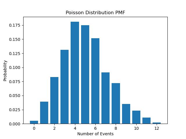
We can see that the probability mass function is right skewed and has a long tail to the right. This means that the probability of observing a large number of events is very small. For example, the probability of observing events is approximately which is very small compared to the probability of observing events, which is approximately .
This visualization can be applied to many real-world scenarios, including modeling the number of cosmic rays detected in a particular time period or the number of supernova explosions observed in a particular region of the sky. By using the Poisson distribution to model such rare events, we can gain insights into the likelihood of these events occurring and make predictions about future observations.
The final code for this section is given below:
import numpy as np
import matplotlib.pyplot as plt
from scipy.stats import poisson

lambda_ = 5

samples = poisson.rvs(mu=lambda_, size=1000)

unique, counts = np.unique(samples, return_counts=True)

plt.bar(unique, counts/1000)
plt.xlabel('Number of Events')
plt.ylabel('Probability')
plt.title('Poisson Distribution PMF')
plt.show()
Properties of the Poisson Distribution
The Poisson distribution has following important properties:
- The Poisson distribution is a discrete probability distribution, which means that it can only take on discrete values. For example, the number of traffic accidents in a day cannot be a fraction, and it can only take on integer values.
- The Poisson distribution is a memoryless distribution, which means that the probability of observing a certain number of events in the future is independent of the number of events that occurred in the past. For example, the probability of observing traffic accidents in a day is independent of the number of accidents that occurred in the previous days.
- The Poisson distribution is a non-negative distribution, which means that it can only take on non-negative values. For example, the number of traffic accidents in a day cannot be negative.
- The Poisson distribution right skewed, which means that the probability of observing a large number of events is higher than the probability of observing a small number of events. For example, the probability of observing traffic accidents in a day is higher than the probability of observing traffic accident in a day.
Poison noise
Poisson noise is a type of noise that arises when counting rare events that follow a Poisson distribution. Poisson noise is the result of the statistical fluctuations of the number of events occurring in a given interval.
For example, in astronomy, Poisson noise is often encountered when counting photons from distant celestial objects. The number of photons detected by a telescope follows a Poisson distribution, and the statistical fluctuations in the number of photons result in Poisson noise. Understanding the level of Poisson noise is important in determining the uncertainty in the measurements, and hence the accuracy of the resulting scientific conclusions.
Example problem
Suppose we have counted a total of 10,000 photoelectrons over a period of 10 minutes from incoming photons at a CCD pixel of an astronomical telescope. What is the noise level or uncertainty in that photoelectron count?
Solution with Python
We can use the Poisson distribution to calculate the uncertainty in the photoelectron count. Since the Poisson distribution has a variance equal to its mean, we can estimate the mean photoelectron count as the total number of photoelectrons divided by the measurement time. In this case, the mean photoelectron count is:
Using this mean value, we can calculate the standard deviation or uncertainty of the photoelectron count as:
Therefore, the Poisson noise or uncertainty in the photoelectron count is approximately 31.6 photoelectrons per minute.
We can also verify this result using Python. Here is an example code snippet that calculates the uncertainty in the photoelectron count using the Poisson distribution:
import numpy as np
from scipy.stats import poisson

total_photoelectrons = 10000
measurement_time = 10 # minutes

mean_photoelectrons = total_photoelectrons / measurement_time
print("Mean photoelectron count:", mean_photoelectrons)

std_photoelectrons = np.sqrt(mean_photoelectrons)
print("Standard deviation or uncertainty:", std_photoelectrons)

# Poisson distribution
poisson_dist = poisson(mu=mean_photoelectrons)

# Probability of measuring exactly the mean value
prob_mean = poisson_dist.pmf(mean_photoelectrons)
print("Probability of measuring exactly the mean value:", prob_mean)
After running the code, we get the following output:
Mean photoelectron count: 1000.0
Standard deviation or uncertainty: 31.622776601683793
Probability of measuring exactly the mean value: 0.01261461134870819
We have used the scipy.stats{:python} module to create a Poisson distribution with the estimated mean photoelectron count, and then calculates the probability of measuring exactly the mean value. The resulting probability is small, indicating that the actual photoelectron count is likely to deviate from the mean value due to Poisson noise.
Conclusion
The poisson distribution is a useful tool for modeling the occurrence of rare events. Its properties, including its mean and variance, make it well-suited for a wide range of real-world applications. From modeling the arrival of customers at a store to understanding the behavior of photons in telescopes, the Poisson distribution has proven to be a valuable tool in many fields. With the help of Python, it is easier than ever to apply the Poisson distribution to real-world problems and gain insights into the behavior of rare events.
